Back to basics: multivariate qualitative analysis, SIMCA

Full-Text PDF

A.M.C. Davies^a and Tom Fearn^b

^aNorwich Near Infrared Consultancy, 75 Intwood Road, Cringleford, Norwich NR4 6AA, UK. E-mail: [email protected]
^bDepartment of Statistical Science, University College London, Gower Street, London WC1E 6BT, UK. E-mail: [email protected]

DOI: https://doi.org/10.1255/sew.2008.a1

Introduction

In our previous column¹ we introduced CVA, one of the very early applications of multivariate analysis (1930s). In this column we will discuss SIMCA (officially it is Soft Independent Modelling of Class Analogies, but no one uses the long form!). SIMCA was invented 30 years later² by another pioneer, Svante Wold (the man who coined the word “chemometrics”).

SIMCA

The idea

When CVA is used with high-dimensional data, some prior reduction of dimension is needed. The standard approach is to combine data from all the groups and apply a single PCA. SIMCA takes a different approach, making separate PCA models for each group. This is indicated in Figure 1. Each group has its own PC space which is normally modelled with only a few PCs (typically two to four). If you compare this figure with Figure 1 in the previous article you will see the immediate difference between SIMCA and CVA.

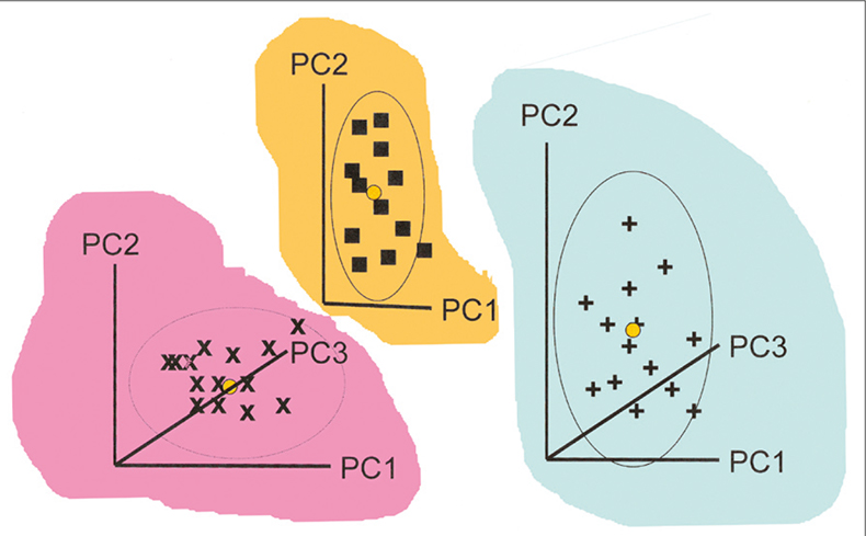
Figure 1. Calculation of individual PCA for three groups of samples for use in SIMCA. The coloured backgrounds indicate that the models may lie in completely different spaces.

Application

When we have a new sample which is believed to be a member of one of these groups we make two calculations comparing the sample to each group and use the results to decide if the sample is likely to be a member of any of the groups. These measurements are a Euclidian distance of the sample to the model (e_i) and a Mahalanobis^* distance within the principal component space (h_i). The calculation is shown diagrammatically, for two groups, in Figure 2.

Figure 2. SIMCA for two groups. (a) Group 1 is modelled by two PCs, PC1(1) and PC2(1) while group 2, is modelled by a single PC, PC1(2). (b) A new sample, O, is compared to each group by projecting it on to the models, a plane in the case of group 1, a line for group 2. This gives the distances ei(1) and hi(1) for group 1 and ei(2) and hi(2) for group 2.

While it may be advantageous to have two measurements, we then have to decide how to combine them. One approach is to apply thresholds separately, i.e. both distances have to be less than chosen cut-off values before the unknown qualifies for group membership, as in the graphs shown below. Another is to combine the distances by squaring them, adding and taking the square root of the sum.^† A single threshold is then applied to this combined distance.

Graphical methods for SIMCA

Because SIMCA uses different PC models for each group, there is no general plot which can be used for looking at all the groups in a single plot. There are two plots which can be used for assessing SIMCA results. The “Coomans’ Plot” compares the distance to the model (e_i) results in pairwise plots; so you have to look at plots for all possible pairs. After those you have to look at the “Membership” plot which plots distance to model (e_i) against the distance from the model centre (h_i) for unknown (test) samples for a selected model. Both of these plots can have limits also plotted to help decide if a sample could be a member of the group. The limits are calculated, using some often rather doubtful distributional assumptions, to exclude a chosen percentage of samples that do actually belong to the group. The higher this percentage (e.g. 25% is used for e_i in the plots below) the less chance that non-members will be assigned to the group. In the Unscrambler SIMCA program that we used for our calculations, the percentage on which the h_i threshold is based is fixed probably at 5% (the manual is not clear on this!) and cannot be varied.

Honey classification

In the previous column¹ we showed CVA results using NIR data of different botanical sources of honey⁴ and now we will use the same data with SIMCA to see if it gives similar results.

Figure 3 shows Coomans’ plots for the six possible pairwise combinations of four groups, applying a 25% significance limit to e_i. Looking at 3(a)^‡ which compares acacia honey (model AcP3) with chestnut honey (model ChP5) (the 3 and 5 in these models indicates the number of PCs). The vertical line is the limit for the sample being likely to be acacia if it is to the left of the line. The horizontal line is the limit for the sample being classified as chestnut if it is below the limit. Samples which fall in the lower left quadrant could be members of either group while samples in the upper right quadrant are classified as not being a member of either group. These calculations are based on very few samples and we had to use cross-validation⁵ (the same samples used for training and testing). It should be emphasised that this is for demonstration only. This data set was a borderline one for CVA because of its size; it is much too small for SIMCA. On this plot the red or blue letters are the sample identity of the cross-validation samples used in calibration while the green letters show the actual membership of test samples (non-members of either group).

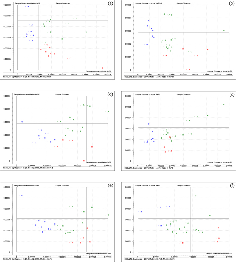
Figure 3. Coomans’ plots of honey samples. (a), acacia v. chestnut; (b), acacia v. heather; (c) acacia v. rape; (d), chestnut v. heather; (e), chestnut v. rape; (f), heather v. rape.

Figure 4 shows the “Membership” plots for the four groups. These are plots of distance to the model (ordinate) and the distance to model centre (abscissa) for each honey group. The limits are again plotted as vertical and horizontal lines. To be confident that a sample could be a member of this group it should appear in the lower left quadrant.

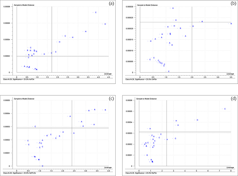
Figure 4. Membership plots for the honey data. (a) Acacia, (b) chestnut, (c) heather, (d) rape honeys.

Interpretation of the honey results

Acacia

Figure 3(a) shows that all the acacia samples are classified as being acacia, six of them could also be chestnut. Figure 3(b) shows that all the samples in the acacia group could be acacia and three of them could be classified as heather. Figure 3(c) shows that all the acacia samples are classified as acacia but five of them could also be rape samples. Figure 4(a) shows that all the acacia samples are classified as acacia and only one sample of chestnut honey could also be incorrectly identified as acacia. These results show that the acacia group are all very similar and are quite well differentiated from the other three groups when both distances are taken into account.

Chestnut

Figure 3(a) shows that the chestnut samples all plot in area for classification as chestnut. None of them is classified as acacia but the majority of the other honeys could be (incorrectly) classified as chestnut. Figure 3(d) has a similar result. All the chestnut samples and most of the other samples are classified as being chestnut or heather. Figure 3(e) also shows similar results; all the chestnut samples are correctly identified but most of the other samples are also classified as rape. Figure 4(b) shows that many honey samples appear in the lower left quadrant and are classified as chestnut but the real chestnut samples form a tight group and their distance values are nearer to the origin than any non-chestnut sample.

Heather

The Coomans’ plots 3b, 3d and 3f indicate that the heather samples do not constitute a well formed group. (Heather honey is notorious for being mixed with honey from other nectars either by the bees, beekeepers or traders.) Two of the samples were so distant that they had to be excluded from the study. Many non-heather samples could be classified as heather. The “Membership” plot, Figure 4(c) shows that the remaining five samples of heather honey do form a characteristic group, apparently at odds with the evidence from the Coomans’ plots.

Rape

The Coomans’ plots indicate that rape is a well classified group but many other honeys are incorrectly classified as rape. The “Membership plot”, Figure 4(d) shows the rape samples are closer to the origin than the other samples classified as rape.

Summary of the results

It would appear from this analysis that acacia and rape can be reliably classified but there is considerable overlap with heather and chestnut samples. Much the same as obtained by the CVA study of the same data but rather harder to tune and interpret.

Comment

For its simplicity we would always choose PCA + CVA as the default method for a spectroscopic classification problem. The main drawback of SIMCA is the difficulty of tuning it: the results can be quite sensitive to the dimensions of the models and the choices of thresholds. However, it does also have advantages, possibly the most useful being that if a new group (a new ingredient for example) comes along, it is possible to add it to the system without starting the whole analysis from scratch.

References

A.M.C. Davies and T. Fearn, Spectrosc. Europe 20(4), 18 (2008). https://www.spectroscopyeurope.com/td-column/back-basics-multivariate-qualitative-analysis-canonical-variates-analysis
S. Wold, Pattern Recogn. 8, 127–139 (1976). https://doi.org/10.1016/0031-3203(76)90014-5
T. Næs, T. Isaksson, T. Fearn and T. Davies, A user-friendly guide to multivariate calibration and classification. NIR Publications, Chichester, pp. 131–133 (2002). https://store.impopen.com/a-user-friendly-guide-to-multivariate-calibration-and-classification.html
A.M.C. Davies, B. Radovic, T. Fearn and E. Anklam, J. Near Infrared Spectrosc. 10, 121–135 (2002). https://doi.org/10.1255/jnirs.329
A.M.C. Davies, Spectrosc. Europe 10(2), 24 (1998).