A.M.C. Daviesa and Tom Fearnb
aNorwich Near Infrared Consultancy, 75 Intwood Road, Cringleford, Norwich NR4 6AA, UK. E-mail: [email protected]
bDepartment of Statistical Science, University College London, Gower Street, London WC1E 6BT, UK. E-mail: [email protected]
The starting point for this column is the last one from last year! In that column TD began what was intended to be a two-part story but has, with this column, become a story in four parts. There were required topics we had not covered and we need to begin this column by completing the discussion of removing multiplicative effects by describing what the two most popular methods do to NIR spectra.
Introduction
The starting point for this column is the last one from last year! In that column TD began what was intended to be a two-part story but has, with this column, become a story in four parts.1–3 There were required topics we had not covered and we need to begin this column by completing the discussion of removing multiplicative effects by describing what the two most popular methods do to NIR spectra.
Multiplicative scatter correction
In 1981, Ian Murray working at the (then) School of Agriculture, Aberdeen, presented a technique for reducing scattering which he called “Mathematical Ball-milling”.4 It was not adopted by any of the instrument software systems, so it did not catch on. In 1985 Geladi, MacDougall and Martens published a similar technique which they called Multiplicative Scatter Correction5 (MSC), which was adopted and has become one of the most used methods of data pre-treatment of NIR data. These were the first new methods to attempt to correct for scatter correction since the work of Kubelka and Munk.6 The idea is that spectra are shifted vertically by scattering but in a multiplicative way; not just by a constant or linear addition.
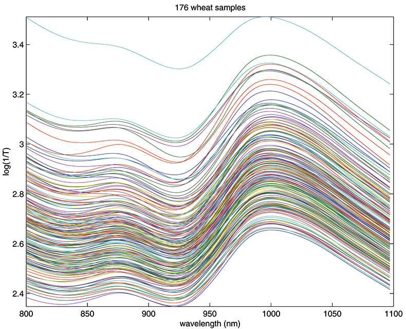
Figure 1. Spectra of 176 samples of whole-grain wheat.
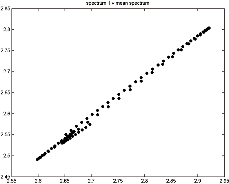
Figure 2. Spectrum 1 versus mean spectrum.
Figure 1 shows 176 transmission spectra, obtained from samples of whole grain using a Tecator Infratec Grain Analyser. The spectral range is 850–1048 nm in steps of 2 nm. The basis for the method is that if you plot the 100 spectral points for sample 1 against the 100 corresponding points of the mean spectrum, as in Figure 2, the result looks roughly like a straight line. MSC fits a straight line to this plot by least squares and uses the slope and intercept of the line to “correct” spectrum 1. If the regression of spectrum 1 on the mean spectrum has intercept a and slope b, and the log(1/T) values for spectrum 1 are x1, x2, ..., x100, then the MSC corrected values are (xi – a)/b for i = 1, ..., 100. Thus spectrum 1 is shifted vertically and scaled proportionally to make it as close as possible to the mean spectrum. This is repeated for each of the 176 spectra in turn, and subsequently for any new spectra that have to be pre-treated. This requires the mean calibration spectrum to be stored along with the calibration equation for prediction purposes, a possible slight drawback to the approach. The effect of MSC on our 176 spectra can be seen in Figure 3.
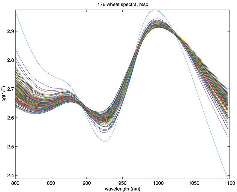
Figure 3. Spectra in Figure1 after MSC.
Standard normal variate
Another equally popular method, which takes a slightly different approach to the multiplicative scattering, is the so-called standard normal variate (SNV) transformation.7 This also shifts and scales each spectrum, but now using coefficients derived from that spectrum alone. For spectrum 1 we calculate the mean, m, and the standard deviation, s, of the 100 log(1/T) values, xi, and transform to (xi – m)/s. The procedure is then repeated for spectrum 2 and so on. This approach has the attraction that we do not need to carry around a mean spectrum to pre-treat unknowns in the future. Since all these means can get confusing, it is perhaps worth emphasising that the mean, m, used here is a mean over 100 wavelengths for one spectrum. The mean spectrum used in MSC is a mean over 176 samples at each wavelength. The effect of SNV on the wheat transmission spectra can be seen in Figure 4.
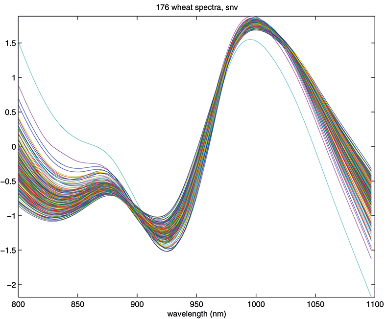
Figure 4. Spectra in Figure 1 after SNV.
The results in Figures 3 and 4 look very similar. This is not surprising because the methods are mathematically related; however, in use they are not quite equivalent, so with one data set MSC will lead to a better calibration than SNV, while with another set the reverse will be true. If you like, you can decide which you prefer and stick to it or you could always evaluate which results in the better calibration. What is certain is that there is no point in using both in the same calibration! Now we can return to our calibration task and see if we can improve on the previous result.1
The calibration task
You will need to have the previous article1 to hand (if you have not retained it you can download a copy from the Spectroscopy Europe website8) but we will repeat the main points. The task is a pharmaceutical calibration. We have a data set (T1) of 460 analysed tablets, which we are using for calibration and a set (C1) of 155 analysed tablets that we are using for validation. The samples were small experimental batches; we also have 40 samples (V1), not mentioned in the previous article, for an additional validation test. These were samples from two production batches of the same formulation (2 × 20). The NIR data was recorded over the range 600–1898 nm at 2 nm intervals. However, in the preliminary study it was decided to use a reduced range of 788–1686 nm. The tablets have been weighed and analysed for a propriety pharmaceutical active coded “assay” (mg/tablet). The tablet weights are required because spectroscopy measures concentrations but patients take tablets so during calibration we work in concentration units but then we need to convert measured (or predicted) concentrations back into dosage per tablet. In the previous article a preliminary calibration gave a result for the root mean square error prediction (RMSEP) for set C1 of 4.78 mg/tablet so now we will iterate with different pre-treatments of the spectra to ascertain if we can discover a calibration which will give an improved RMSEP. As we will be guided by plots similar to those previously shown, only a few will be repeated.
Results
In each iteration, we attempt to optimise each calibration by excluding some high influence samples and determining the number of PLS factors to use by using half of the calibration set as a test set. Figure 5 is a typical “Influence” plot which indicates a few samples that have a large effect on the calibration which is undesirable and so we can remove them. It is important to note that this is a desirable and correct procedure for calibration data as the calibration may be improved but it should not be done for validation samples. This just fools us into believing that the calibration has improved; it has not!
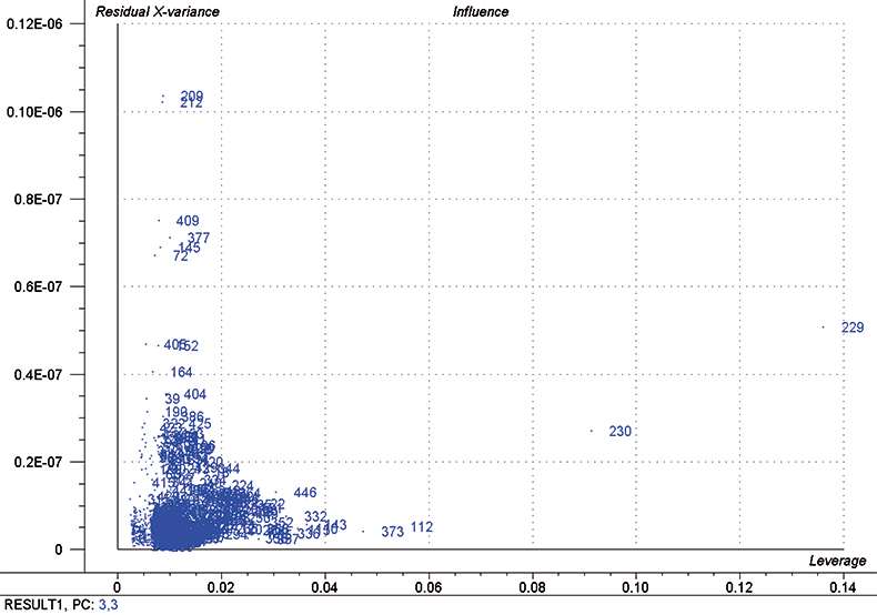
Figure 5. Influence plot; samples 112, 229, 230 and 373 were removed from the final calibration.
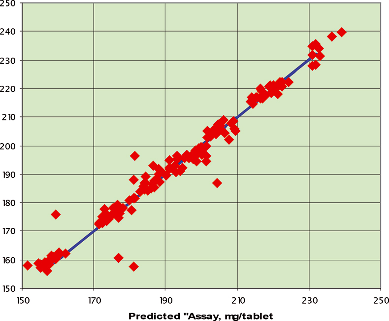
Figure 6. Prediction results for the C1 data set; RMSEP=3.94 mg/tablet.
Table 1. Results for prediction of dosage in pharmaceutical tablets using various data pre-treatments.
Test number | Pre-treatment | Calibration RMSCEV on T1 | Number of PLS factors | Prediction RMSEP on C1 |
1 | None | 1.10 | 3 | 4.54 |
2 | Second derivative (d2, 3, 5) | 0.93 | 3 | 3.94 |
3 | MSC | 0.93 | 3 | 4.09 |
4 | SNV | 1.11 | 2 | 5.14 |
5 | Test 2 + MSC | 0.92 | 3 | 4.07 |
6 | Test 2 + SNV | 0.91 | 3 | 4.06 |
The final calibration for each iteration was computed from the complete T1 calibration set using cross-validation and the calibration was tested on set C1. All these procedures were in concentration units; to make the final assessment the prediction results were converted to dosage using the provided tablet weights (weight of active per tablet) and compared to the given analyses. Table 1 lists the results for various pre-treatments. Compared to the previous results we see that with the reduced variable range no pre-treatment gives quite a good calibration which is better than SNV on its own. The second derivative computation gave a slightly lower RMSEP on C1 validation samples and so this is our preferred calibration. Figure 6 is a plot of the results for validation of this calibration. Now that we have a final selected calibration it will be interesting to see how well it predicts the V1 production samples. The result was an RMSEP of 1.95 mg/tablet, which is a pleasing result. However, we have not quite finished! If we plot the V1 results against sample number, Figure 7, we can see that there is a difference between the two batches. The first 20 samples have an average of 193.7 while the second 20 samples have an average of 197.0. The power of NIR data analysis is even more striking if we look at the plot for these samples in the Unscrambler program, Figure 8. These results are in concentration units but the large difference between the two batches is the Unscrambler calculation of deviations of the predictions. The larger the box the more uncertain the result. There is clearly something very different about the second batch of production samples. If they had these results being produced in real time perhaps the line controller could have discovered the cause?
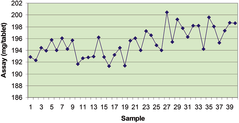
Figure 7. Prediction results for the V1 production tablets plotted against sample number.
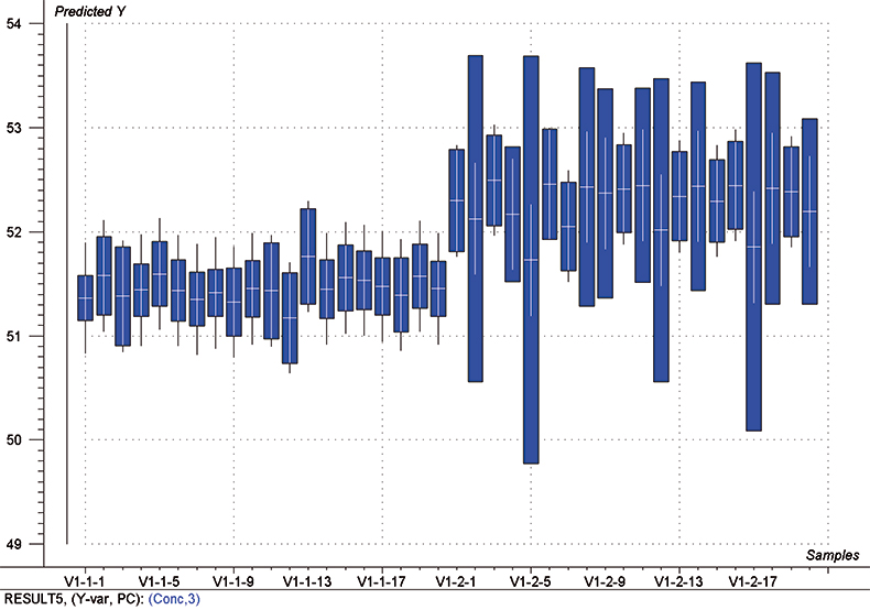
Figure 8. Prediction results (concentration) for the V1 production samples. The boxes indicate the uncertainty of the results; the larger the box the more uncertain the result.
Conclusion
You cannot learn how to do multivariate calibration from this one example, but we hope it will give people who have never attempted such a task to have a go. The data is still available on the IDRC website.9 You will get different results, ours are slightly different from those obtained by David Hopkins,10 there may be a much better calibration waiting to be found—by you!
References
- A.M.C. Davies, Spectroscopy Europe 18(6), 28 (2006).
- A.M.C. Davies, Spectroscopy Europe 19(2), 32 (2007).
- A.M.C. Davies and T. Fearn, Spectroscopy Europe 19(4), 24 (2007).
- I. Murray, C. Jessiman and H. Kenley, 12th Annu. Meet Eur. Soc. Nuci. Methods Agric. (1981).
- P. Geladi, D. MacDougall and H. Martens, Appl. Spectrosc. 39, 491 (1985).
- P. Kubelka and F. Munk, Z. Techn. Physik 12, 593 (1931).
- R.J. Barnes, M.S. Dhanoa and S.J. Lister, Appl. Spectrosc. 43, 772 (1989).
- https://www.spectroscopyeurope.com/td-column/back-basics-running-your-first-pls-calibration
- www.idrc-chambersburg.org/shootout_2002.htm
- D.W. Hopkins, NIR news 14(5), 10 (2003).