A.M.C. Davies
Norwich Near Infrared Consultancy, 75 Intwood Road, Cringleford, Norwich NR4 6AA, UK
Introduction
In my last column I began a revision of basic chemometrics.1 In this column I will discuss some interpretation of the results produced by principal component analysis (PCA) as part two of this revision programme.
Understanding PCA is one of the best introductions into the world of chemometrics where we invent new variables from combinations of old variables and rotate data to discover more useful views of its structure. The study of PCA could be justified solely to gain these insights but in fact it is one of the most useful tools in the chemometric toolbox!
Looking at data structure
I am going to use an excellent example demonstrating PCA, which originates from my friends Tormod Næs and Tomas Isaksson.2 They took three chemicals, casein, glucose and calcium lactate and made all possible mixes at 5 % variation as indicated by Figure 1.
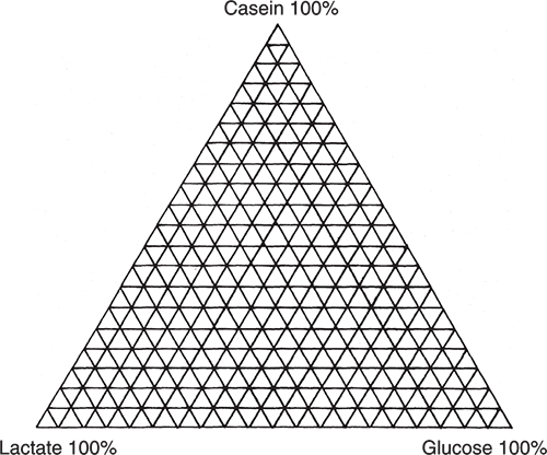
Figure 1. Experiment design for producing mixtures of casein, glucose and lactate. Each vertex corresponds to a sample.
Then they measured the NIR spectra of all 231 mixtures. The NIR spectra were corrected for scatter using multiplicative scatter correction and then entered into a PCA program. The scores plot in Figure 2 is for the first two principal components (PCs). It is very obvious from the triangular distribution of the samples that the two plots are connected. In fact the data has been flipped and rotated! You can see this because of the labels and you could also check it by knowing the identities of the extreme samples (each should be due to a 100 % pure ingredient) but we can also check the information via the loadings. There are some areas where the distribution is not quite perfect. This might be due to very small errors in weighing or less than optimal mixing. It might also be due to some interactions between the ingredients. These areas would need to be subjected to further experimentation to see if the variations were stable when repeated with additional samples prepared with new weighings and mixing. However, this is not our present interest but it is another insight into the information content of scores plots. They really are very useful. Our interest is to understand how PCA has achieved this result and the way we do that is to compare the spectra and the loadings of the PCs.
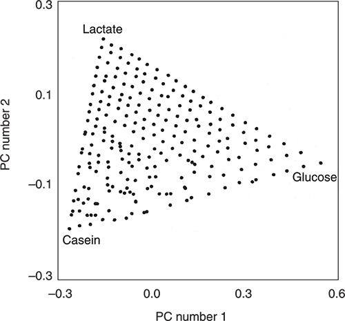
Figure 2. The PCA scores plot produced from the scatter-corrected NIR spectra of the 231 mixtures.
Figures 3 to 5 are the spectra of the pure ingredients. If we believe that the labels on Figure 2 are correct then we see that PC1 is mainly measuring increase in glucose so we would expect to that the PC1 loadings would be similar to the glucose spectrum. However, there is something that we need to remember from the earlier column; the first operation in PCA is to centre the data (mean centring). So rather than look at the glucose spectrum we must look at the glucose minus the mean spectrum of the 231 spectra. This is shown in Figure 6 and below it in Figure 7 is the loadings plot of PC1. The two plots do look pleasingly similar.
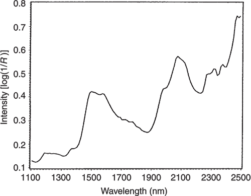
Figure 3. The NIR spectrum of pure glucose.
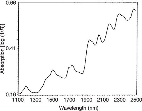
Figure 4. The NIR spectrum of pure casein.
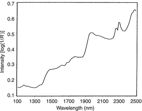
Figure 5. The NIR spectrum of pure lactate.
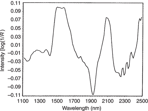
Figure 6. The mean-centred spectrum of glucose.
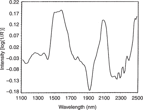
Figure 7. The loadings plot for PC1.
If we look at the loadings plot for PC2 in Figure 8 it looks much more complex than the spectra of either casein or lactate. The answer is to think about what is happening when we move in the PC2 direction in Figure 2. We are moving from high casein concentration to high lactate concentration and this suggests that the PC2 direction is related to a difference in the concentration of these two constituents. If we compare the PC2 loading plot in Figure 8 with the difference between the casein and lactate spectra in Figure 9 we again find a surprising agreement. Well I find it surprising, so I hope you do!
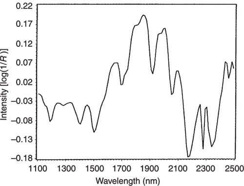
Figure 8. The loading plot for PC2.
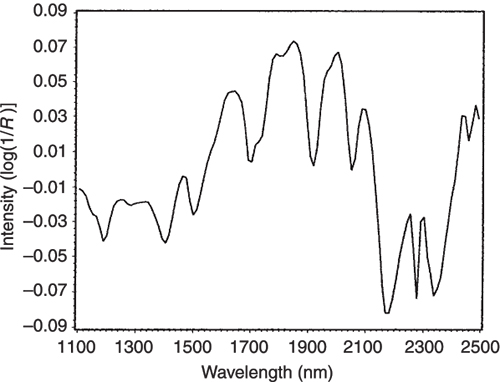
Figure 9. The difference between the NIR spectra of the pure casein and lactate samples.
Conclusions
This is of course a near perfect, designed experiment; with real-life samples it may be not so clear cut and you may have to test different interpretations to find the most likely one. You will also have realised that PCA does not just discover the underlying spectra of the pure compound so that again in real-life situations you do need to be cautious about your interpretations and be prepared for the unusual to happen. Having given that warning, I can finish by assuring you that this is a very useful technique that really does work and can provide crucial chemical information. That is the purpose of chemometrics!
Acknowledgements
I am very pleased to be able to thank Tormod and Tomas for the use of their data. I had discussed the outline of this column with Tom Fearn but he has recently been unwell and now he is recovered but on holiday. As he has not had the opportunity to check the column I am reluctant to add his name to it; I might have made some terrible mistake that he will be blamed for! Instead I would like to acknowledge all the help he gives me with many of these columns and all that I have learned from him, over many years, that I attempt to pass on to you!
References
- A.M.C. Davies, Spectroscopy Europe 16(6), 20 (2004).
- T. Næs and T. Isaksson, NIR news 3(3), 7 (1992).
Note
A similar account of this data has been published in the book:
T. Næs, T. Isaksson, T. Fearn and T. Davies, A User-Friendly Guide to Multivariate Calibration and Classification. NIR Publications, Chichester (2002). https://doi.org/10.1255/978-1-906715-25-0