Jean-Sébastien Dubé, ing. PhD and François Duhaime, ing. PhD
Laboratoire de géotechnique et génie géoenvironnemental, Département de génie de la construction, École de technologie supérieure, 1100 Notre-Dame ouest, Montréal (QC), Canada H3C 1K3
Proper sampling of particulate matter for instrumental analysis is a common task in many applied scientific, technology and engineering fields. It is a crucial task for ensuring that measurements made on a given set of samples are representative estimate of the parameters of interest in the original sampling target. Unfortunately, sampling particulate matter is in many fields performed without a scientific basis, mostly because its critical role is ignored, or at best, misunderstood, and because of an unawareness of, sometimes a disregard for, the Theory of Sampling. This two-part column illustrates this important point using experience in the field of geo-environmental engineering.
Environmental site assessment guidelines require representative sampling, but do not define how: a recipe for decision-making disaster
A noteworthy example of how sampling is performed without a proper scientific basis is the sampling involved in environmental site assessment of contaminated soil. In this context, soil samples are analysed for their content of contaminants (chemical, physical). For chemical contaminants, analytical protocols generally require a few grams of soil for analysis only, and specify that this small quantity must be representative of the field parcel from which it is derived. This implies that a few grams of soil must represent a volume up to several hundred cubic metres of particulate matter in the field. This implies a mass reduction of nothing less than six to nine orders of magnitude, while ensuring that at each stage of the mass reduction process the resulting sub-sampled quantity of matter still represents the entire original soil parcel. With the current state-of-affairs in this field (guidelines, standards, tradition, ignorance) this is a well-nigh impossible task. We find it incumbent upon us to sound a serious alarm within the field of geo-environmental engineering—but the examples and lessons described below have a much wider impact in many applications fields with similar heterogeneity issues.
The representativeness of an analytical measurement, i.e. the degree to which it represents the real contaminant content in the soil, compositionally as well as spatially, is directly related to the representativeness of the sampling process. This means the degree to which the proportion of each type of constitutive element of the soil, particles and contaminant(s) is preserved during the “from-field-to-analysis” sampling/sub-sampling process.
However, in the vast majority of current cases, the degree of representativeness is not assessed, far less even mentioned. In most guidelines for sampling of contaminated soils, representativeness is a vague concept, mostly owing to some form of wishful thinking. Without a formal definition of representativeness and guidelines on how to obtain a desired degree of sampling representativeness (called “fit-for-purpose representativity”), sampling is performed more or less intuitively, haphazardly or based on subjective judgement. This approach is called grab sampling in the Theory of Sampling (TOS). It most commonly involves taking the desired mass of soil (“not-too-much”) from some accessible part of the soil in one increment. In today’s practice in the field, this would result in a grab sample of a few hundred grams which is sent to the laboratory, where a grab sub-sample of a few grams is then taken for analysis.
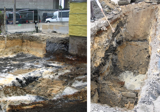
Typical test pits in geo-environmental engineering site soil characterisation. One attribute rules the day: “significant heterogeneity”. It is obvious that any single field sample (a grab sample in the TOS parlance) will not be able to represent the entire site. For this job, diligent compliance with the TOS’ principle of composite sampling is necessary (see part 2).
Below are two realistic, real-world examples of how this approach to sampling can produce extremely poor results.a
Assessment of zinc contamination
The first example is typical of a common situation in the practice of environmental assessment. A field sample from a site contaminated with zinc (Zn) was sent to an analytical laboratory by a geo–environmental consultant charged with the environmental assessment study. Field and laboratory sampling were performed by grab sampling. As per common practice, the laboratory was charged with providing a single analytical result from the material in the container delivered. This measurement resulted in a Zn concentration of 1900 mg kg–1, thus indicating a contamination well above the regulation threshold for the current usage of the site (see further below). This result would lead to the demand that the soil from the parcel must be removed.
However, several in situ semi-quantitative measurements were also made by the consultant on the soil parcel with the use of a portable X-ray fluorescence spectrometer, and these had indicated a possibly smaller concentration.
Therefore, the consultant asked the laboratory for “a second measurement” based on the same sample container. This time the results came in at 79 mg kg–1. Such a major discrepancy “naturally” prompted a third measurement, which, however, failed to detect any Zn in the soil! At the end of a very confusing day, a total of seven individual measurements were made based on the same 300 g soil sample as shown in Table 1.
Table 1. “Autopsy” of a single 300 g field soil sample, and the resulting soil remediation status (categorisation).
Measurement | Concentration (mg kg–1) | Categorisation based on measurement |
1 | 1900 | >III |
2 | 79 | <I |
3 | <4 | <I |
4 | <4 | <I |
5 | <4 | <I |
6 | 700
| II–III |
7 | 25 | <I |
I, II and III represent regulatory thresholds of 140, 500 and 1500 mg kg–1, respectively.
Que faire?
As a way of trying to shift the burden of explaining these wildly varying results to the consultant, the laboratory concluded that the sample received was not homogeneous. Although this conclusion is correct, such a conclusion is profoundly naïve as all soils are heterogeneous, it is only a matter of to which degree (TOS).
This self-evident truth was exacerbated in the present case by severely “incorrect” sub-sampling in the laboratory (grab sampling from the same field sample container). So, whatever heterogeneity was revealed only pertained to the scale of the volume of the field container. Whether this is the same heterogeneity characterising the significantly larger site volume under investigation is still a completely open question: how well does the field container represent the entire site?
The applicable regulatory thresholds were 140 mg kg–1 (I), 500 mg kg–1 (II) and 1500 mg kg–1 (III), each value representing the maximum allowed Zn concentration in soil for specific usages of the site, or specific means of disposal of the excavated soil. Table 1 also shows the categorisation of the soil with respect to these thresholds based on each of the seven “replicated” measurements.
It comes as no surprise that the consultant was now confronted with the confounding problem of correctly categorising the soil parcel represented by one field sample, but seven analytical results. If the categorisation decision had been made based on a single measurement, as is the usual practice, a highly significant error would have been introduced. This would have transferred unwarranted significant uncertainty to the site remediation process. The key issue is, of course, that under “normal practices” this would not even have been known to any of the stakeholders involved.
It would be hazardous to fit a statistical distribution to such a small dataset in which 43 % of the data are left censored. However, it is possible to roughly estimate the categorisation probabilities based on proportions as shown in Table 2.
Table 2. Estimates of categorisation probabilities (categories A, B, C are identical to categories I, II, III in Table 1).
Category | Probability |
x<A | 0.714 |
A<x<B | 0 |
B<x<C | 0.143 |
x>C | 0.143 |
If the consultant had used the first measurement, as in current practice, he would have categorised the soil as larger than criterion III and, therefore, in need of disposal off site (A). But the probability that this decision would have been correct is only 14.3 % (Table 2).
The consultant was, therefore, well advised to ask the laboratory for supplemental measurements. While these vary widely, a Kaplan–Meier (KM) estimate of the mean Zn concentration, 388 mg kg–1,b indicates that the soil could be categorised as being lower than criterion III, and thus kept on the site. This decision would have had an 85.7 % probability of being correct. The problem of categorising the soil becomes more acute when the soil must be excavated and disposed of off site, since the disposal cost is related to the contamination level category. In the present case, based on the singular initial measurement, the soil would have been categorised as larger than criterion III, and disposed of at a larger cost, most probably incurring unnecessary expenditures from the site owner. However, based on the KM mean of 388 mg kg–1, the soil would have been categorised as between criteria I and II, and thus disposed of at a much smaller cost or even reused as fill material in some jurisdictions. This example illustrates well how much uncertainty can be introduced in the decision-making process if based on a single 300 g field soil sample.
It can come as no surprise then that the documented uncertainty points to the highly likely situation that the target lot from which this single field sample originated must be significantly heterogeneous itself. The key issue is: is the single field sample representative of this target lot? To answer that, attention must be directed elsewhere: how was the primary sample (the field container) sampled in the field? Were the principles and rules in the TOS complied with, or not?
The situation depicted is common and typical, but it is not acceptable. The only way such a problematic situation can be improved upon is by invoking a stronger focus on the characteristics of the full sampling process, notably the primary field sampling stage.
This case is also “representative” of the ill-informed practice of pouring more money into the analysis stage, i.e. making a larger number of measurements from each primary sample. Instead, more care should be taken in reducing variability at the primary sampling stage. It should not be difficult to understand that the debilitating heterogeneity revealed in Table 1 is only a reflection of the state-of-affairs in the singular field sample upon arrival at the analytical laboratory. No manner of repeated analysis based on this sample alone, can produce any information as to the real-world heterogeneity of the entire soil parcel, which must be larger but to an unknowable degree. The obvious solution is an appropriate deployment of composite sampling covering the entire 3-D parcel site.
Preliminary conclusion, Part 1
The first part of the full sampling-and-analysis process occur in the field and is often performed by the consultant’s field technician. This gap in the “chain of custody” of the sampling process between the consultant and the laboratory is particularly problematic, especially as much as the current incorrect sampling practices are left without a clear responsibility. No one takes full responsibility for the representativeness of the complete sampling process in such circumstances.
Fix your sampling, not your results
In part 2 we will further illustrate how measurement variability can be controlled at the sampling stage with a second real-world example from a recent study conducted at École de technologie supérieure, Montréal, in partnership with the same consultant involved in the first example presented here. In this second study, we compare the uncertainty derived from grab sampling to that derived from a TOS-compliant composite sampling process.
Footnotes
aFor the record: the examples and procedures discussed here pertain to significantly heterogeneous materials that cannot be subject to mixing before sampling. If a significantly heterogeneous lot to be sampled happens to be so small that it is economically feasible to mix it thoroughly in its entirety, the rules of the game have been altered because mixing leads to a significantly reduced distributional heterogeneity. However, the resultant lot is still compositionally heterogenous and still needs to be treated as such. Such cases are exceedingly rare, and consequently of overwhelmingly little interest within geo–environmental engineering.
bNote that calculating the mean Zn concentration by arbitrarily substituting the censored concentration measurements, i.e. <4 mg kg–1, by 0 or 4, we obtain a mean Zn concentration ranging from 383 mg kg–1 to 388 mg kg–1. While these estimates of the mean are close to the KM estimate in this case, arbitrary substitution in environmental datasets can lead to unreliable and biased estimates of descriptive parameters). Dennis Helsel (doi.org/fdmnj8) comments on arbitrary substitution: “There is an incredibly strong pull for doing something simple and cheap”. This statement can just as aptly also be applied to grab sampling at all stages from field to aliquot.
References
A complete list of References will be included in part 2.
Testimony
Understanding what sampling variation is, and how it is estimated, has been a “light-bulb” moment for our analysts after having been introduced to the Theory of Sampling (TOS) principles. So often we have had a situation where analytical work and results can be verified, but our customer still insists it doesn’t meet expectations. Short of driving the poor analyst crazy with re-work tasks, which usually only produces the same “incorrect result”, I now have an avenue of action that allows us to guide the customer and analysts to the path on how to focus on only taking representative samples. This is decidedly more welcome than always having to hear: “Take the sample back to the lab—repeat the analysis”.
Much time is spent determining the combined total uncertainty for specific analytical methods under validation, however, very little attention is given to the preceding sampling errors and the challenges heterogeneity poses to this issue. I now know that sampling errors dominate over their analytical cousins. Also, using variographic characterisation as a quality control tool for process and measurement system monitoring is a very powerful technique that could help process controllers explain the sources of real process variations that occur on their product lines instead of simply following through by blaming the analytical lab. I found that the new international standard DS 3077 (2013) and in particular its use of illustrations and industrial examples captured the true complexity of the principal types of sampling errors and helped to conceptualise the TOS principles in a strikingly visual way, making it easier for a typical chemical analyst to relate to the scenarios involved before analysis. After all, we have to isolate the absolutely smallest aliquot for analysis—as demanded by highly sophisticated analytical instrumentation. It is, therefore, highly surprising that the one area of greatest error affecting analysts’ results is the same topic largely ignored in Analytical Chemistry/Science Training programmes, again the sampling errors. This gives rise to “brilliant” analytical results, i.e. extremely precise results, but for non-representative samples for which accuracy with respect to the lot is not accounted for. In fact the accuracy of the analytical results with reference to the original lot is completely without control—and one cannot even estimate the magnitude of the sampling bias incurred (because it is inconstant, as is another insight provided by TOS). This makes for a very unsure analytical laboratory. After this course I wonder how many questionable results have been released by laboratories all over the world over many, many decades—and the revelations brought about by TOS are still not known!
Dr Melissa C. Gouws, InnoVenton Analytical, Port Elizabeth, South Africa
Reproduced from K.H. Esbensen, Introduction to the Theory and Practice of Sampling. IM Publications Open, Chichester, UK (2020) with permission. ©2020 IM Publications Open LLP